Simple AutoEncoder
Here I’ll describe second step in understanding what TNNF can do for you. Using MNIST data - let’s create simple (one layer) sparse AutoEncoder (AE), train it and visualise its weights. This will give understanding of how to compose a little bit complicate networks in TNNF (two layers) and how sparse AE works.
Data
To train our AE - let’s use widely known MNIST data set.
You can download it in .csv format here: http://www.pjreddie.com/projects/mnist-in-csv
As .csv format is comparatively slow and increases train time significantly we recommend to use HDF to store data on your drive.
It takes you to install h5py package to start use it. Here is more about it.
Note
It’s better to download their package instead of trying to install through pip.
Once you install h5py you need to convert .csv to HDF. I’ve prepared a short script in Python for you to do this.
You can download it directly from GitHub. You need to run it against both .csv files: train and test sets.
Here is what you need to change there:
srcFolder = './src/'
csv_type = '.csv'
hdf_type = '.hdf5'
target_csv = 'mnist_test'
target_hdf = 'mnist_test'
- Where:
- srcFolder - directory, where csv file locatedcsv_type - .csv file extension. You don’t need to change it usually.hdf_type - HFD file extension. You don’t need to change it usually.target_csv - .csv file name, without extension.target_hdf - HDF file name. File will be created and filled with data from .csv .
After all you will have two .h5py files with train and test MNIST data.
Mini batches
Using whole data we have is usually computationally ineffective. Moreover, in modern task it is impossible. We can gather millions (or billions) of examples for our training, so we will face with memory issue even for data storage. To address this issue people usually use mini batches. In other words, instead of training algorithm on the whole available data - we train algorithm on the number of randomly sampled examples from the whole data set. We call such examples - mimibatch. Be aware, examples should be sampled randomly from whole dat set into the miniBatch.
To speed up training time, we will use miniBatches. To sample each batch we will use small function included in the example code:
#Sampling minibatch from whole data set
def getBatch(d, n, i):
    idx = random.sample(i, n)
    idx = np.sort(idx)
    #Remove labels and read data
    res = d[idx, 1:]
    #Normalise output from 0..255 to 0..1
    return res.T / 255.0
- Where:
- d - HDF data set
- n - number of batches to sample
- i - list of valid data’s indexes to sample from
Theory
A little theory about sparse constraint, how it looks like.
When we introduce sparse constraint to our network, we expect that average activation of particular neuron for one data’s batch will be equal to the one, we specified. To achieve this - we will add penalty to the network error each time our real average activation will diff from the specified. To estimate, how big this penalty should be we use Kullback-Leibler equation. Here how it looks like:
To be more human oriented, let’s visualise its graph.
On the following graph we assume we want our average activation = 0.2 . Then, given variety of average activation on X-axis we can observe penalty value on Y-axis.
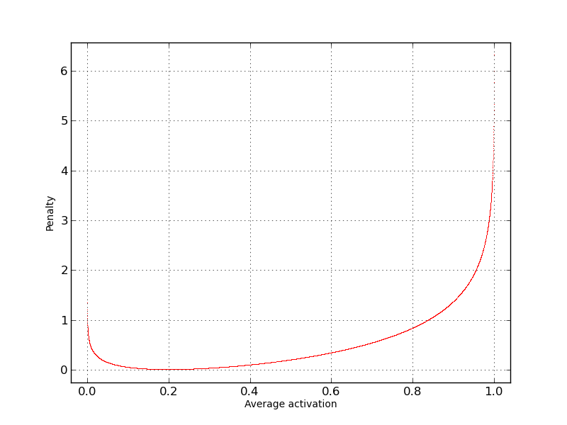
As you can see - Penalty is very close to zero only when our Average activation is close to the 0.2 and vice-versa - the more average activation gets away from desired 0.2, the bigger Penalty becomes.
We will restrict hidden layer average activation to force neural network detect common patterns in input data. Concretely, we restrict the number of neurons we need to describe data. This means, that every neuron that activates - represents pattern (features) in input data.
Neural Network
We done with theory, let’s program AE using TNNF!
So our AE consist of two layers and has Input, Hidden and Output abstracts. Don’t be confused with three abstracts. Input abstract is always there. It doesn’t take separate layer.
As input we have 28x28 images, that gives us 28 x 28 = 784 values for each example on the input. As we train AE, the neural network that tries to replicate on the output what it has on input - we have 784 values on output.
Let’s use 196 neuron on the hidden layer with average activation = 0.1 . (Architecture took from UFLDL tutorial)
Everything above give us next network architecture:
- Input: 784 neurons
- Hidden: 196 neurons (with average activation restricted to 0.1)
- Output: 784 neurons
To represent this in code we need two layers. First layer:
L1 = LayerNN(size_in=inputSize,
             size_out=numberOfFeatures,
             sparsity=0.1,
             beta=3,
             weightDecay=3e-3,
             activation=FunctionModel.Sigmoid)
- Where:
- size_in - 784 (number of neurons on the input)
- size_out - 196 (number of neurons on hidden layer)
- sparsity - 0.1, average hidden layer activation we want to achieve
- beta - sparsity coefficient (how strong we amplify sparsity penalty)
- weightDecay - weight penalty (just to improve training time, you can try to run without it)
- activation - activation function to use (calculating sparsity constraint makes sense only for Sigmoid)
Second layer:
L2 = LayerNN(size_in=numberOfFeatures,
             size_out=inputSize,
             weightDecay=3e-3,
             activation=FunctionModel.Sigmoid)
- Where:
- size_in - 196 (number of neurons on hidden layer, we use first layer output as input to the second)
- size_out - 784 (number of neurons on output equal to the input)
- weightDecay - weight penalty (again, just to improve training time, you can try to run without it)
- activation - activation function to use (calculating sparsity constraint makes sense only for Sigmoid)
Be default, script will do the following:
- assume that HDF data files are located in: script directory/Data/src (you can change this in the script)
- train set file name: mnist_train.hdf5
- test set file name: mnist_test.hdf5
- perform 10,000 iterations
- use miniBatch size of 200 examples per batch
- check cross validation (CV) error every 500 iterations and print it
- print square error and square error + all penalty each iteration
- save error vs iterations graph every 500 iterations in the script’s directory
- save hidden layer weights visualisation in the script’s directory
On laptop GPU GeForce GT 635M it takes about 3 minute to finish. On laptop CPU i5-3210M CPU @ 2.50GHz (on numpy 1.9.1 and OpenBLAS recompiled to use all cores) it takes about 8 minutes.
Parameters we use to run tests:
THEANO_FLAGS=mode=FAST_RUN,floatX=float32,device=gpu python ScriptName.py
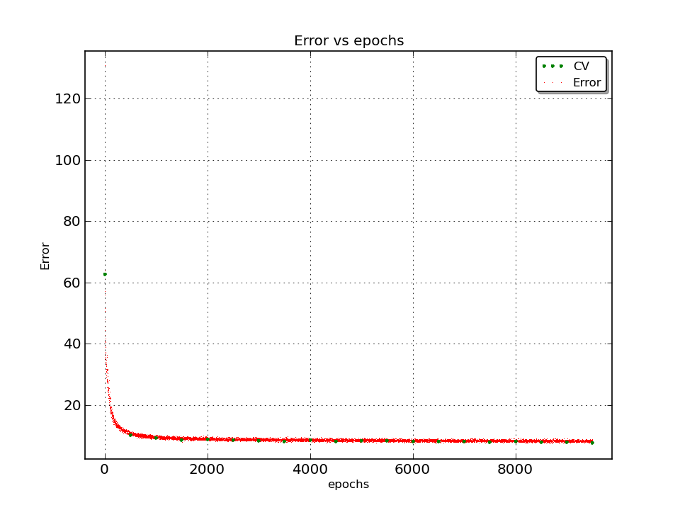
How AE error evolves with iterations:
To inspire you and add some clearness what AE is and how its weights evolves through the time we prepared and added cool gif visualisation. It is ~5 Mb, so it takes some time to load.
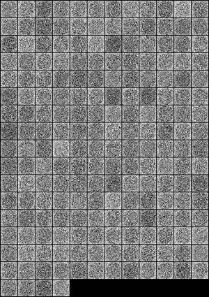
Final features (hidden layer’s weights) in the original size:

Full SimpleAutoEncoder script listing:
import numpy as np
import unittest
import os
import sys
import h5py
import random
sys.path.append('../../../CORE')
from fTheanoNNclassCORE import OptionsStore, TheanoNNclass, NNsupport, FunctionModel, LayerNN
from fGraphBuilderCORE import Graph


#Sampling minibatch from whole data set
def getBatch(d, n, i):
    idx = random.sample(i, n)
    idx = np.sort(idx)
    #Remove labels and read data
    res = d[idx, 1:]
    #Normalise output from 0..255 to 0..1
    return res.T / 255.0

#We use HDF because of its speed and convenience
#Set data's file names and path
srcFolder = './Data/src/'
hdf_type = '.hdf5'
train_set = 'mnist_train'
test_set = 'mnist_test'

#Read train data
f_train = h5py.File(srcFolder + train_set + hdf_type, 'r+')
DATA = f_train['/hdfDataSet']

#Read CV data
f_test = h5py.File(srcFolder + test_set + hdf_type, 'r+')
DATA_CV = f_test['/hdfDataSet']

#Print out shapes of loaded data
print 'Data shape:', DATA.shape, '\n', 'CV shape:', DATA_CV.shape

#Extract some useful data
dataSize = DATA.shape[0]
cvSize = DATA_CV.shape[0]
validDataIndexes = xrange(0, dataSize)

# As we have all data we need for Auto Encoder (AE),
# let's create an appropriate NN

# Set few additional options
numberOfFeatures = 196
batchSize = 200
inputSize = DATA.shape[1] - 1   # Subtract label
iterations = 10000
checkCvEvery = 500

#Common options for whole NN
options = OptionsStore(learnStep=0.005,
                       rmsProp=0.9,
                       mmsmin=1e-20,
                       minibatch_size=batchSize,
                       CV_size=cvSize)

#First layer
L1 = LayerNN(size_in=inputSize,
             size_out=numberOfFeatures,
             sparsity=0.1,
             beta=3,
             weightDecay=3e-3,
             activation=FunctionModel.Sigmoid)

#Second layer
L2 = LayerNN(size_in=numberOfFeatures,
             size_out=inputSize,
             weightDecay=3e-3,
             activation=FunctionModel.Sigmoid)

#Compile all together
AE = TheanoNNclass(options, (L1, L2))

#Compile train and predict functions
AE.trainCompile()
AE.predictCompile()

#Normalise CV data from 0..255 to 0..1
X_CV = DATA_CV[:, 1:].T / 255.0

#Empty list to collect CV errors
CV_error = []

#Let's iterate!
for i in xrange(iterations):

    #Get miniBatch of defined size from whole DATA
    X = getBatch(DATA, batchSize, validDataIndexes)

    #Train on given data/labels
    AE.trainCalc(X, X, iteration=1, debug=True, errorCollect=True)

    #Check CV error every *checkCvEvery* cycles
    if i % checkCvEvery == 0:

        #Caclculate CV error give CV data/labels
        CV_error.append(NNsupport.crossV(X_CV, X_CV, AE))

        #Print current CV error
        print 'CV error: ', CV_error[-1]

        #Draw how error and accuracy evolves vs iterations
        Graph.Builder(name='AE_error.png', error=AE.errorArray, cv=CV_error, legend_on=True)

        #Visualise hidden layers weights
        AE.weightsVisualizer(folder='.', size=(28, 28))