Simplest example¶

Data
Neural Network
How it performs

I’ll try do describe how to use TNNF to solve a simplest artificial task I was able to design.

Let’s create a simple classifier that will assign 0 or 1 class to data from input. And as we don’t want random classification, let’s try to train our classifier on previously manually labeled data.

Data¶

Let’s imagine we have some amount of manually labeled data (to label data we will use particular “decision rule”). This data will be used to train our classifier.

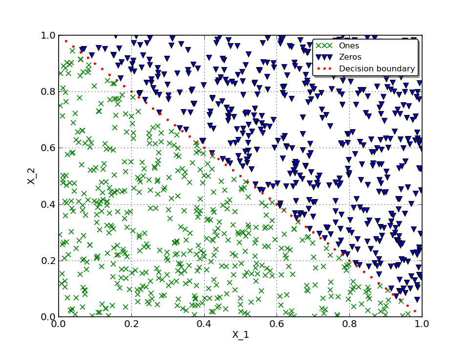
In this particular task I assume we have to classify a pair of numbers \((X_1, X_2)\), where \(X_1, X_2 \in [0, 1)\) and assign each pair 0 or 1 class. To manually label this data let’s use such formula:

\[\begin{split}Label = \begin{cases} 0 & \text{if: } -X_1 + 1 < X_2\\ 1 & \text{if: } -X_1 + 1 \geq X_2 \end{cases}\end{split}\]

Here is how our labeled data looks on 2D plot:

Neural Network¶

As was mentioned - let’s use TNNF to solve this task.

What we have:

Randomly generated data for training
Randomly generated data for cross-validation
Labels

What we want to achieve:

Given generated data - using TNNF - predict correct labels

To do this, we will use one-layer Neural Network with simplest Linear activation function and architecture:

Input layer: 2 neurons
Output layer: 1 neuron

To define predicted label we will round the activation of output layer:

\[\begin{split}Output = \begin{cases} 0 & activation \leq 0.5\\ 1 & activation > 0.5 \end{cases}\end{split}\]

Here is how it looks in code.

Set general options for whole network, such as:

Learning step
Size of mini-batch we will use (in this case we use full batch)
Size of cross-validation set

#Common options for whole NN
options = OptionsStore(learnStep=0.05,
                       minibatch_size=dataSize,
                       CV_size=dataSize)

Describe per layer architcture. Set:

Number of neurons on layer’s input
Number of neurons on layer’s output
Specify activation function to use

#Layer architecture
#We will use only one layer with 2 neurons on input and 1 on output
L1 = LayerNN(size_in=dataFeatures,
             size_out=1,
             activation=FunctionModel.Linear)

Put everything together and create network object:

#Compile NN
NN = TheanoNNclass(options, (L1, ))

How it performs¶

Instead of talking how well it performs its better to show this. To visualise predicted boundary we will use network’s weights and bias that it learned during training.

As we use Linear activation function, we can write a formula to calc output activation:

\[activation = w_1X_1 + w_2X_2 + b\]

Using our previous formula to define predicted label, we can rewrite this as follows:

\[w_1X_1 + w_2X_2 + b \gtreqless 0.5\]

To be able to draw predicted decision boundary we need to express \(X_2\) :

\[X_2 \gtreqless -\frac{w_1}{w_2}X_1 + \frac{0.5 - b}{w_2}\]

Here is how it looks like in code:

        #Recalculate predicted decision boundary
        y_predicted = -w1 * x / w2 + (0.5 - b) / w2

If you enable drawing and set reasonable drawEveryStep you will get number of pictures that shows how Neural Net evolves. To get rid you from routine we already did this with small drawEveryStep and prepare a gif to show a progress:

As you can see - with each iteration Neural Net moves closer to original decision boundary. That is what we wanted to show you: how Neural Network adapt and learn on real data.

Here is one more informative graph. We can track how accuracy and network error evolves vs iterations.

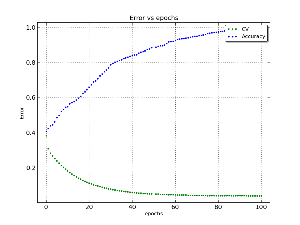
It almost reach 100% accuracy!

Full script listing:

import numpy as np
import unittest
import os
import sys
sys.path.append('../../../CORE')
from fTheanoNNclassCORE import OptionsStore, TheanoNNclass, NNsupport, FunctionModel, LayerNN
from fDataWorkerCORE import csvDataLoader
from fGraphBuilderCORE import Graph
from matplotlib.pylab import plot, title, xlabel, ylabel, legend, grid, margins, savefig, close, xlim, ylim

dataSize = 1000
dataFeatures = 2

#Supposed boundary line
#Where x - [0] row, f(x) - [1] row in data
# if f(x) < -x + 1 - then label = 1
#                    else label = 0

#Create random data [0, 1)
data = np.random.rand(dataFeatures, dataSize)

#Create random cross-validation [0, 1)
CV = np.random.rand(dataFeatures, dataSize)

#Create array for labels
labels = np.zeros((1, dataSize))

#Create array for cross-validation labels
CV_labels = np.zeros((1, dataSize))

#Calc labels (and cross-validation) based on supposed boundary decision function analytically
labels[0, :] = -data[0, :] + 1 > data[1, :]
CV_labels[0, :] = -CV[0, :] + 1 > CV[1, :]

#Let's draw our data and decision boundary we use to divide it
#Calc decision boundary
x = np.arange(0, 1.0, 0.02)
y = -x + 1

#Draw labeled data
#Uncomment next part if you want to visualise input data
'''
ones = np.array([[], []])
zeros = np.array([[], []])
for i in xrange(dataSize):
    if labels[0, i] == 0:
        zeros = np.append(zeros, data[:, i].reshape(-1, 1), axis=1)
    else:
        ones = np.append(ones, data[:, i].reshape(-1, 1), axis=1)

xlim(0, 1)
ylim(0, 1)

plot(ones[0, :], ones[1, :], 'gx', markeredgewidth=1, label='Ones')
plot(zeros[0, :], zeros[1, :], 'bv', markeredgewidth=1, label='Zeros')
plot(x, y, 'r.', markeredgewidth=0, label='Decision boundary')
xlabel('X_1')
ylabel('X_2')

legend(loc='upper right', fontsize=10, numpoints=3, shadow=True, fancybox=True)
grid()
savefig('data_visualisation.png', dpi=120)
close()
'''

#Check average
avgLabel = np.average(labels)

print data.shape
print 'Data:\n', data[:, :6]
print labels.shape
print 'Average label (should be ~ 0.5):', avgLabel

#For now we have labeled and checked data.
#Let's try to train NN to see, how it solves such task
#NN part

#Common options for whole NN
options = OptionsStore(learnStep=0.05,
                       minibatch_size=dataSize,
                       CV_size=dataSize)

#Layer architecture
#We will use only one layer with 2 neurons on input and 1 on output
L1 = LayerNN(size_in=dataFeatures,
             size_out=1,
             activation=FunctionModel.Linear)

#Compile NN
NN = TheanoNNclass(options, (L1, ))

#Compile NN train
NN.trainCompile()

#Compile NN oredict
NN.predictCompile()

#Number of iterations (cycles of training)
iterations = 1000

#Set step to draw
drawEveryStep = 100
draw = False

#CV error accumulator (for network estimation)
cv_err = []

#Accuracy accumulator (for network estimation)
acc = []

#Main cycle
for i in xrange(iterations):

    #Train NN using given data and labels
    NN.trainCalc(data, labels, iteration=1, debug=True)

    #Draw data, original and current decision boundary every drawEveryStep's step
    if draw and i % drawEveryStep == 0:

        #Get current coefficient for our network
        b = NN.varWeights[0]['b'].get_value()[0]
        w1 = NN.varWeights[0]['w'].get_value()[0][0]
        w2 = NN.varWeights[0]['w'].get_value()[0][1]

        #Recalculate predicted decision boundary
        y_predicted = -w1 * x / w2 + (0.5 - b) / w2

        #Limit our plot by axes
        xlim(0, 1)
        ylim(0, 1)

        #Plot predicted decision boundary
        plot(x, y_predicted, 'g.', markeredgewidth=0, label='Predicted boundary')

        #Plot original decision boundary
        plot(x, y, 'r.', markeredgewidth=0, label='Original boundary')

        #Plot raw data
        plot(data[0, :], data[1, :], 'b,', label='data')

        #Draw legend
        legend(loc='upper right', fontsize=10, numpoints=3, shadow=True, fancybox=True)

        #Eanble grid
        grid()

        #Save plot to file
        savefig('data' + str(i) + '.png', dpi=120)

        #Close and clear current plot
        close()

        #Estimate Neural Network error (square error, "distance" between real and predicted value) on cross-validation
        cv_err.append(NNsupport.crossV(CV_labels, CV, NN))

        #Estimate network's accuracy
        accuracy = np.mean(CV_labels == np.round(NN.out))
        acc.append(accuracy)

        #Draw how error and accuracy evolves vs iterations
        Graph.Builder(name='NN_error.png', error=NN.errorArray, cv=cv_err, accuracy=acc, legend_on=True)